3) Two phenotypes

This example demonstrates how to incorporate multiple phenotypes into the cosegregation analysis. It also showcases how the app can deal with consanguineous families.

Pedigree table

The data corresponding to the case is shown below:

 ped id fid mid sex phenotype carrier proband age
   1  1   0   0   1         .       .       .  50
   1  2   0   0   2         .       .       .  50
   1  3   1   2   1         .       .       .  50
   1  4   0   0   2      mild       .       .  50
   1  5   1   2   1         .       .       .  50
   1  6   0   0   2    nonaff       .       .  50
   1  7   3   4   1    severe     het       .  50
   1  8   0   0   2    nonaff       .       .  50
   1  9   5   6   1      mild       .       .  50
   1 10   0   0   2    nonaff       .       .  50
   1 11   7   8   1    nonaff       .       .  50
   1 12   9  10   2      mild     het       .  50
   1 13  11  12   1    severe     het       1  50
   1 14  11  12   2      mild     het       .  50
   1 15  11  12   2    nonaff     neg       .  50

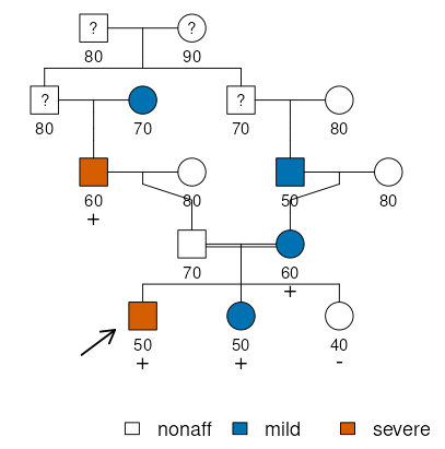
In this family, there are two disease phenotypes: one relatively mild and common, and one more rare and severe. It is hypothesized that the rare autosomal variant found in some members (indicated by + or –) could be associated with increased risks for both. Henceforth, we will assume complete dominance.

Simplified models

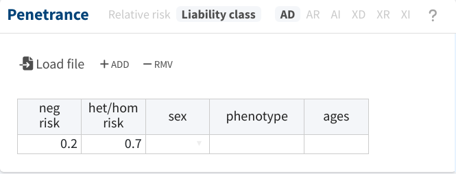
Initially, we will disregard onset/censoring ages by switching to the Liability class mode and declaring age-independent classes.

The most basic strategy would be to also disregard the distinction between both phenotypes and treat both as the same. For instance, let’s say that we suspect the phenocopy rate and penetrance for the mild phenotype to be 20% and 70%, respectively, and we decide to apply these values to all pedigree members:

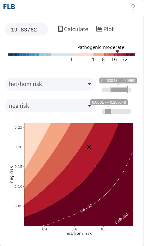
With this setup, we would obtain moderate evidence for pathogenicity, as shown below. The sensitivity analysis also indicates that increasing the ratio of the penetrance-to-phenocopy rate would increase the evidence.

However, we should account for the differences between both phenotypes, if they exist. Luckily, this can be easily done by adding more liability classes and specifying the cases to which they apply. For instance, in the following, we set a phenocopy rate and penetrance for the severe phenotype of 1% and 25%, respectively. Notice that now we also need to specify the parameters for the “unaffected” phenotype (nonaff), which refer to the risk for any of the disease phenotypes.

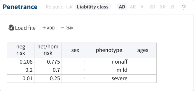
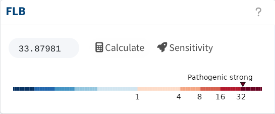
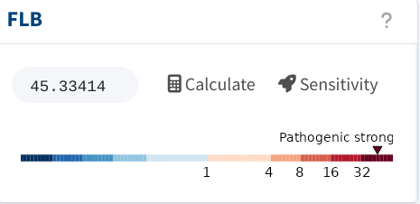
And with that, the FLB shoots to FLB = 45.3, resulting in strong evidence for pathogenicity.

Accounting for ages

Now, let’s complicate the model by considering the ages (of onset or censoring) shown below each pedigree member. This can be done by declaring age-specific liability classes, but it can quickly get cumbersome. To do it, we will switch back to the Relative risk mode.

In this mode, we cannot overlook the distinction between both phenotypes; we must specify the parameters for both. In the following, we use the same risk values (now referring to lifetime risks) as before. Additionally, we consider that phenocopies have an expected onset at 75±20 years of age for the mild phenotype and 60±15 years for the severe one. Notice that for the former, we also specify that the risk conferred by the variant is higher at middle ages; the hazard ratios section of the manual details how to do this.

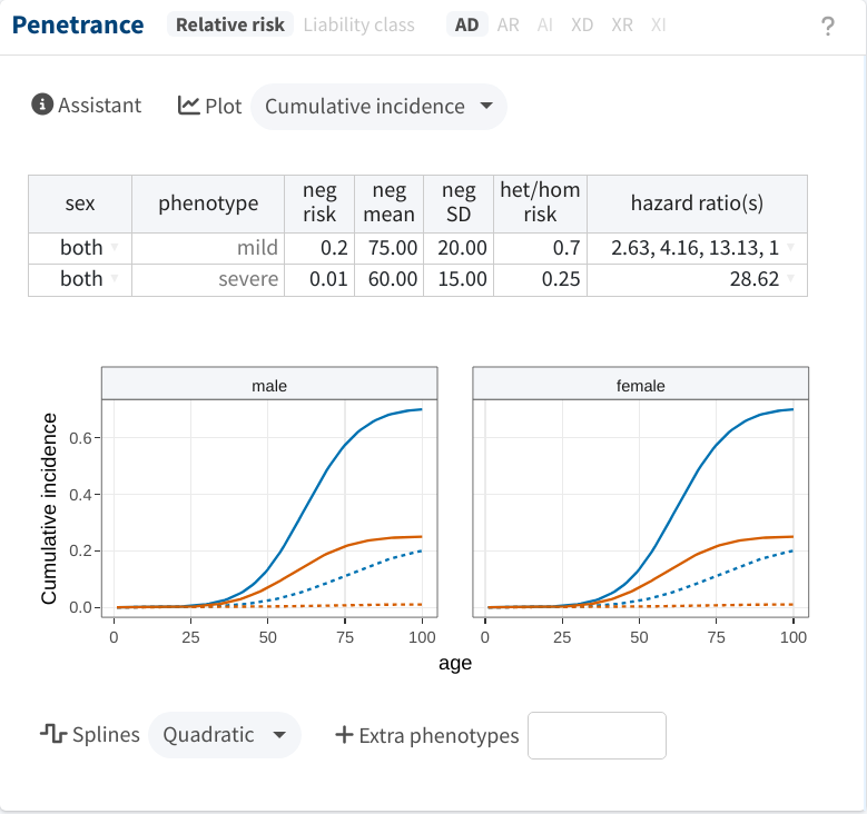
After accounting for the age data, cosegregation evidence is considerably reduced, but it remains strong (FLB > 32).