4) Breast cancer and BRCA1
This example is directly taken from Belman et al. (2020). It puts to the test shinyseg’s more advanced capabilities by requiring a penetrance model with age-dependent relative risks and the explicit declaration of unobserved phenotypes.
Pedigree table
The data corresponding to the case is shown below:
 ped id fid mid sex phenotype carrier proband age
   1  1   0   0   1    nonaff       .       .  80
   1  2   0   0   2      BrCa       .       .  65
   1  3   1   2   2      BrCa     het       .  81
   1  4   1   2   1    nonaff       .       .  41
   1  5   0   0   2         .       .       .  89
   1  6   0   0   1    nonaff       .       .  80
   1  7   1   2   2    nonaff     het       .  75
   1  8   1   2   2    nonaff     neg       .  60
   1  9   4   5   2      BrCa     het       .  41
   1 10   4   5   2      BrCa     het       .  50
   1 11   4   5   2    nonaff     het       .  52
   1 12   6   7   2      BrCa     het       1  49
   1 13   6   7   1    nonaff     het       .  36
   1 14   6   7   2      BrCa     het       .  48
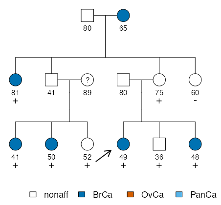
Notice that, together with breast cancer (BrCa), the legend includes
ovarian (OvCa) and pancreatic cancer (PanCa), even though these are
not present in any of the members of the pedigree. This is because they
are still relevant for computing the penetrances and must be included in
the analysis. The next section explains how to do so.
Penetrance
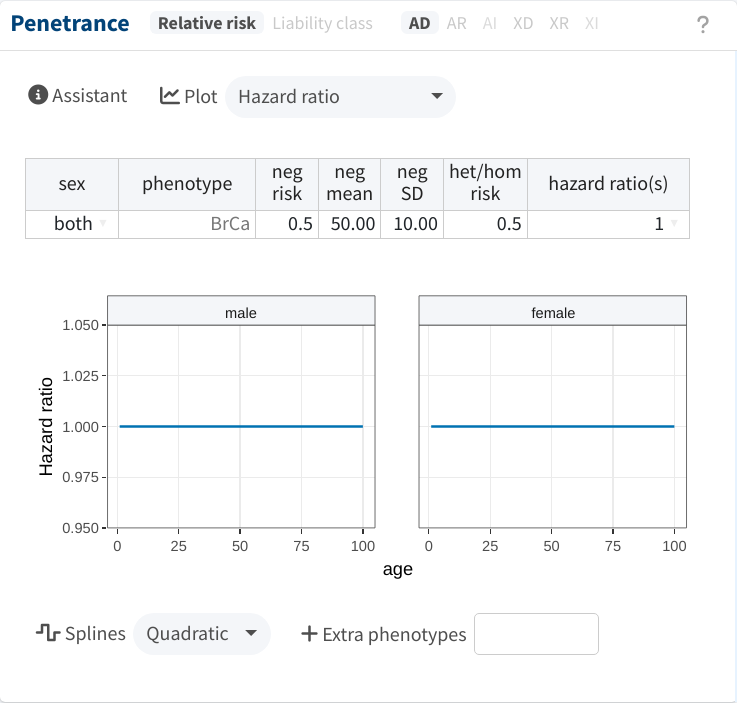
This analysis employs the default Relative risk mode and autosomal
dominant (AD) inheritance. When uploading the previous data to the
app, the relative risk table will only allow parameter setting for
breast cancer, as it’s the sole observed phenotype. It will also consist
of a single row applying to both sexes.
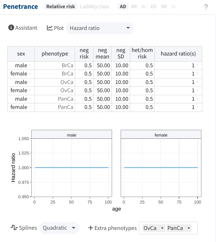
However, in this case involving breast cancer and BRCA1, it is important
to incorporate other cancer types to accurately calculate the
penetrance. This can be achieved by entering their names into the
Extra phenotypes input, located at the bottom of the Penetrance
panel. Moreover, we need to declare sex-specific penetrances. This can
be easily done by clicking on the cells of the sex column and changing
both to any of the sexes. With that done, the table will appear as
follows:
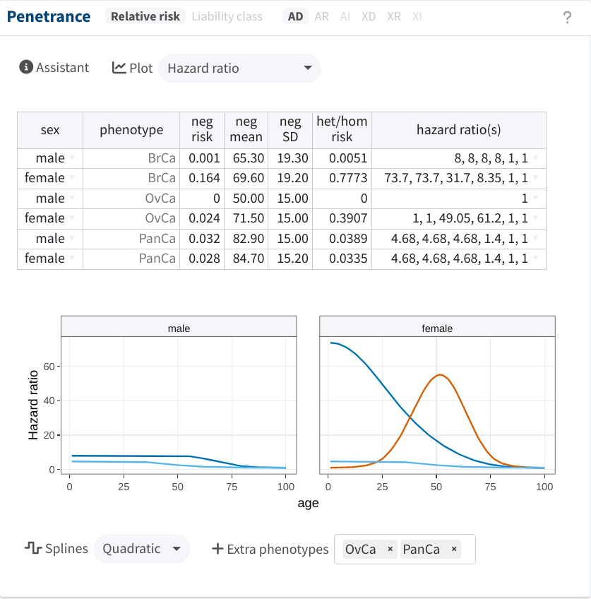
We are now ready to start filling in the table, using the same sources as in Belman et al. (2020):
-
For the baseline parameters (
neg risk,neg mean,neg SD), we employed the UK 2008-2012 estimates from Cancer Incidence in Five Continents (CI5). The optimal parameters for each cancer type were identified by using shinyseg’s Assistant. -
The
hazard ratios(s)were adapted from COOL’s website. We specified the hazard ratios at ages approximately 1, 20, 40, 60, 80, and 100, which are then interpolated/smoothed by the app as shown below.
FLB
Finally, we can Calculate the Bayes factor, which in this case
points to inconclusive evidence for pathogenicity. While this
conclusion aligns with that of Belman et
al. (2020), we note a slight
quantitative deviation (5.7 vs. 3.9) which is primarily due to how
shinyseg utilizes model-based estimates instead of the raw data.

The payoff of shinyseg’s set up is that sensitivity analyses can now be easily performed by altering a reasonable number of parameters.